Linearization of the counts
We had an interesting discussion with an investigator, the opportunity to increase the sampling rate, using an ADC hardware from 500 ksps 13 bit. The intent of this investigator is to count the pulses, Although they are very close together. His goal is to get to 10,000 cps (compared with about 1000 current CPS).
In fact there is no precise point at which you can no longer count, but a gradual increase in the probability of overlapping of impulses (Pileup). We did some tests and we have verified that up to 100 CPS linearity is great, to 500 CPS is beginning to test a significant number of collisions.
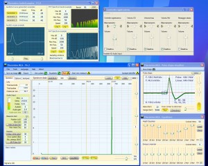
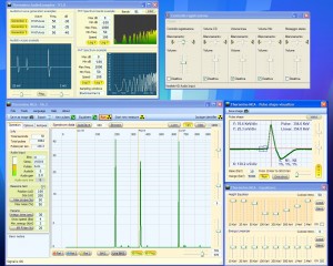
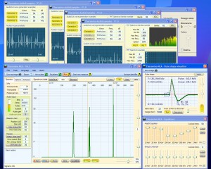
In the following pictures you can see the simulated pulse test (the Simulator produces wide pulse pulse 150 us similar to those of our PmtAdapter)
- Left image 1 impulse 50 times per second, total 50 CPS
- Central image 3 pulses 50 times per second, total 150 CPS
- Right image 10 pulses 50 times per second, total 500 CPS
The pulses measured in these three examples are close enough to 50, 150 and 500 CPS theorists but may change if you go out and light up some test generators. When you turn on a generator that takes a new random location in the pulse train. Two generators exactly overlaid can count by one and repeat the mistake all cycles, but this would not happen with the random data from a PMT.
You may continue until 1000, 5000 and even up to 10000 CPS, but with a gradual progressive loss of pulses (loss of linearity in the upper part of the display range)
A 10000 CPS pulse number lost, would be very high (about 90% and beyond) but it could be compensated, taking into account the progressive increase of probability of collision. The statistical formula is simple and produces a precise linearity correction. (those interested in implementing it finds in the sources of ThereminoGeiger – search for all instances of: “Deadtime”)
Linearize the response with statistical methods degrades performance resolution and sensitivity and is therefore better than acting by brute force on hardware (for example, increase the speed of the ADC or use a sample-hold)
– – – – – – –
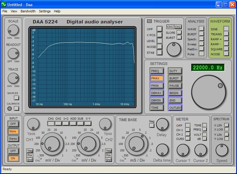
These interesting tests they brought our attention to the bandwidth that, in all sound cards is limited to about 22 kHz. The minimum sampling rate would then 44 kHz (Nyquist law), but internally implement cards over-sampling, sometimes x 2 (and are then defined by 96 kHz) sometimes x 4 (and are therefore to be 192 kHz). In all cases the data is then interpolated to 192 kHz, generating pulses with very gradual trend. And that is exactly what it takes, to measure the exact peak of the pulse.
Here you can see the frequency range of sound cards, ranging from 10 Hz to 22 kHz.
If we use an ADC without bandwidth throttling, We should still integrate data, until soft pulses, to be able to accurately measure.
Without integration, the noise would be very high, because the overwhelming bandwidth. You would lose the opportunity, to see the isotopes of low energy and also the sensitivity and resolution, would be reduced.
– – – – – – –
Focus heavily on sampling frequency, at the expense of everything else, It's not a good idea. In the best case, you could increase the counts to a maximum of two, three, or at best, ten times, but in practice it would not be enough, Let's make some examples:
Earthquake sensing networks have the same problem, all Geophones near catastrophic events, saturate and their data is simply discarded.
If you use sensors can withstand these events, You should discard the same, due to the strong measurement errors caused by the discontinuity that occur near the epicenter.
In the case of earthquakes, the discontinuities are due to fractures of the soil and localized discontinuity caused by rocks and sand. In case of power plant explosion, as Fukushima and Chernobyl, the discontinuities are due to screening of relatively large fragments, torn from the stone bars.
The larger fragments fall into an area of tens of kilometres, making it completely unreliable all sensors in that area. Sand a fragment, such as the one found by Bionerd23 in a flowerbed (www.youtube.com/watch?v = ejZyDvtX85Y), crash sensor, This will measure the highest values, respect in the surrounding area.
You may have huge measurement errors (even 100 times), few meters. La mixture of isotopes would be completely altered, Depending on the composition of the fragment.
– – – – – – – – –
Take for example the German environmental network, based on 1800 Geiger sensors, spaced, on average, ten kilometers away from each other. In the event of a catastrophic event, You should discard four or even ten sensors, but the remaining 1790 provide data, that extrapolated, would make it possible to define exactly the radioactivity to the epicenter.
Quadratic attenuation law, results are much more accurate than what could be discarded sensors.
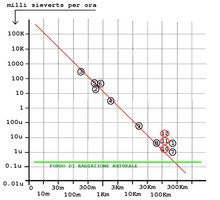
The following image is part of an article we posted after the accident Fukushima, based on data published in 15 days after the explosion the reactor 3.
– PDF document: Probability-and-Risks
– Decumento ODT for translators: Probability-and-Risks
(1) 15/03/2011 in Tokyo 3 micro-sievert per hour ( 10 times the natural radiation background )
(2) 15/03/2011 “the input of the control unit” 11.9 Milli-sievert per hour
(3) 15/03/2011 “near the three-reactor” 400 Milli-sievert per hour
(4) 17/03/2011 measured from helicopters 4.13 Milli-sievert from 1000 feet in height ( 1600m )
(5) 17/03/2011 measured from helicopters 50 Milli-sievert from 400 feet in height ( 640m )
(6) 17/03/2011 measured from helicopters 87.7 Milli-sievert from 300 feet in height ( 480m )
(7) 18/03/2011 measured radiation level in Tokyo about 1 micro-sievert per hour
(8) 18/03/2011 to 60 kilometers from the Central 6,7 micro-sievert per hour.
(9) 18/03/2011 to 20 kilometers from the Central 80 micro-sievert per hour.
(10) 18/03/2011 at Ibaraky 140 kilometers from the Central 2.5 micro-sievert per hour.
(11) 20/03/2011 at Ibaraky 140 kilometers from the Central 6.7 micro-sievert per hour.
(12) 21/03/2011 at Ibaraky 140 kilometers from the Central 12 micro-sievert per hour.
Data published by “Ministry of Education” (www.mext.go.jp), from “Nuclear Safety Division (www.bousai.ne.jp/eng) and from the town of Fukushima, After the helicopter flights.
In this picture you can notice three things:
- Quadratic attenuation law is fully respected. (minimum errors compared to sensor errors)
- The data are extrapolated up near the event.
- You can define the value of radioactivity up to few meters the explosion with great precision.
Also note the location of measuring points closest to the explosion and their values, They also perfectly respected by extrapolation.
– – – – – – –
With a network of thousands of stations you could get a great accuracy, but in an effort do not discard data from any sensor, you degrade the quality of the entire network. Rather it would be better to proceed in the opposite direction and try to decrease noise and maximize the sensitivity and isotope separation.
With Nai(TL) the resolution is always scarce and there is the real possibility of measuring an isotope in place of another. More resolution decreases, the greater this risk.
Linearization of energies
Theremino MCA uses a similar to Equalizer equalizers to linearize the energies and the amplitudes of graphs.
Many expressed doubt that this method is less accurate than that of points with selectable power (Parametric equalizer) used, for example,, in version 6 the PRA.
So you must explain the reason for this choice.
Linearize arbitrary points, unevenly distributed along the spectrum, can produce unnatural curves and big mistakes.
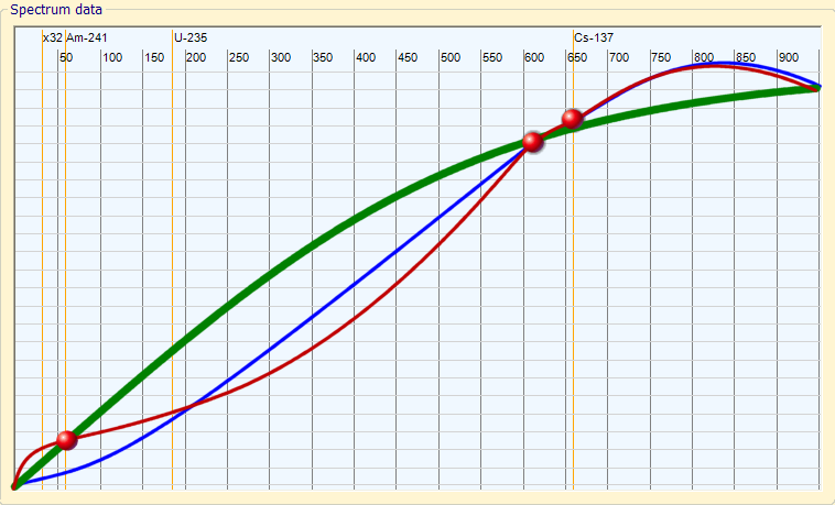
GREEN: The best linearisation curve, that minimizes errors.
BLUE: The linearization curve which is achieved by correcting “almost” exactly the 609 and the 662 Kev
RED: The final curve, After correcting “exactly” even the 59 Kev
“Italian language” – Big mistakes made by a linearization system “accurate” —————————————————————————————————————————————————————— 1) The user corrects “exactly” a peak of Cs-137 in 662 Kev (with a sample of caesium)
2) The user corrects “exactly” a peak of Bi-214 in 609 Kev (with a sample of radio)
3) Because of the inaccuracy introduced by large FWHM of the rows, and also because the number of bin is not infinite, those “accurate” fixes are not so “accurate”
4) Since the distance between the two points of correction (609 and 662) is small, every little inaccuracy extrapolates a big mistake on the entire curve of correction.
5) The user tries a sample of Am-241 in 59,536 Kev, turns out a big mistake, and corrects “exactly” the peak.
6) The user tries a sample of Co-60 in 1.3 MeV, turns out a big mistake, and corrects “exactly” This error.
7) The user now is very happy, all 4 samples are “exactly” correct and linearity is absolutely perfect …. true?
No! The curve “invisible” result is more like a snake to a curve in the real world. Only the points in 59, 609, 662 and 1300 Kev are exactly correct, all other energies are wrong, and with more errors than they would have without the use of any correction. All future analysis made by this “happy user” detect with “accuracy” isotopes that can only be found on samples from the planet Mars.
“English language” – Great errors produced by a “precise” linearization method —————————————————————————————————————————————————————— 1) The user corrects “exactly” a Cs-137 peak at 662 Kev (using a cesium sample)
2) The user corrects “exactly” a Bi-214 peak at 609 Kev (using a radium sample)
3) Because of the imprecision introduced by the large FWHM of the rows, and because the bin number is not infinite, those “exact” corrections are not so “exact”
4) Since the distance between the two correction points (609 and 662) is little, every little imprecision extrapolates a great error on the entire correction curve.
5) The user tests a Am-241 sample at 59.536 Kev, discovers a great error, and corrects “exactly” the 59 KeV peak
6) The user tests a Co-60 sample at 1.3 MeV, discovers a great error, and corrects “exactly” this error
7) The user now is very happy, all the 4 samples are “exactly” corrected and the linearity is absolutely perfect…. is it true ?
No! The “invisible” resulting curve is more similar to a snake, than to a real world curve. Only the points at 59, 609, 662 and 1300 KeV are exactly corrected, all the other energies are wrong, and with more errors than before of this “linearization” All the future analisys made by this “happy user” will find with “precision” isotopes that can be found only on samples coming from Mars planet.
Overfitting
Su Wikipedia si può leggere un’ottima spiegazione di questo effetto: http://en.wikipedia.org/wiki/Overfitting
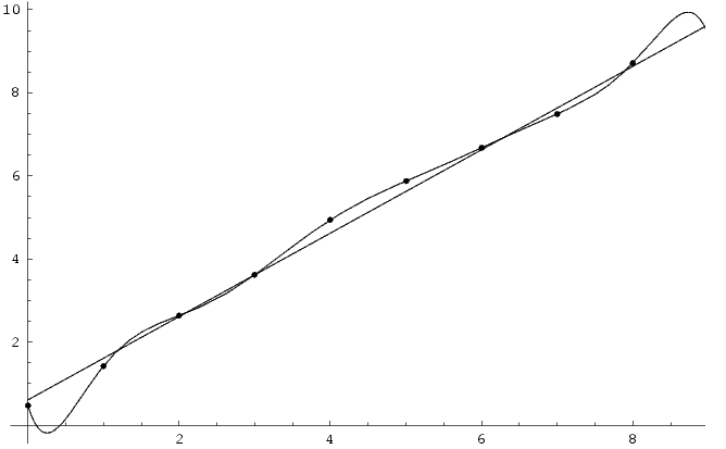
Wikipedia mostra questa immagine e spiega molto bene che:
ITALIANO: Sebbene la funzione di linearizzazione passi esattamente per tutti i punti si otterrebbe un miglior risultato con una retta.
ENGLISH: Although the polynomial function passes through each data point, the linear version is a better fit.


The user Kalin has written to me today with some question about equalizers. They are interesting questions so I decided to copy them here for all the users.
> Kalin <> …there is big difference between using audio equalizers to improve
> the sound of music and using them to calibrate spectrum:
> music is “detected” by ear and its reproduction/perception
> depends on equipment, room ,ambient noise, personal preferences
> and mood :-) So if you give a DJ table with 10 equalizers to two people
> to adjust, they’ll never set them at the same levels (in effect producing
> different output) and I am sure there will be extremes ;-)
Yes, true!
But we are not using true audio equalizers, only the “graphical concept of them”
to facilitate a precise and easy regulation (see the head of this blog)
> Kalin <> On the other hand, in our field we try to match a signal peak to a
> table of relatively precise numbers that do not depend on anything (by
> definition when calibrating with Cs-137 source we trust that say
> Cs-137 has a peak at 660 Kev). In that respect providing analog
> controls (equalizers) may not be the the most straightforward
> approach, although it may work with 1 or 2 point calibration (but try
> it with Eu-152).
To correct Eu-152 ( 121.782 Kev ) we will use the slider marked 100 Kev
it is true that it is not “exactly” at 121,782 but we must correct well
the whole “curve”, non the “single point” energy, so it is better
to use logarithmic spaced correcton points as you can read in the head of this blog.
> Kalin <> May be a good compromise will be to provide text input boxes above
> each equalizer?
This “parametric equalizer” you propose, like the PRA_V6 equalizer, is a good idea
that makes happy all the precision-maniacs, but this method introduces the real risk
to produce big, and invisible, sistematic errors, via the mechanism explained in the
head of this blog
> Kalin <> I am not exactly sure what you mean… Are you saying it will use 5 of
> the peaks (which if there is more that 5?) to calibrate?
With the 5 peaks of the Ra-226 we can calibrate all the spectrum
from 1 KeV to 3 MeV, with a single click, with great precision.
(using equally spaced and logarithmic correction points we hope to reach
not more than 0.5% error in the whole spectrum)
> Kalin <> May be people my age or above have, but I bet younger (say 20ies) had
> very little exposure to those :-)
Each computer program like WindowsMediaPlayer, Winamp, VLC Media Player,
FruityLoops, GarageBand, GoldWave etc.. has a “Graphical Equalizer” so I think
that 99% of the computer users understands this metaphor and knows how to use it.
Per linearizzare le energie pensavamo di usare il Radio (RA-226) It produces four points pretty recognizable with her children:
– PB-214 (241.910 Kev, 295.200 Kev and 351.900 Kev
– BI-214 (609.318 Kev)
Then Happynewgeiger I wrote that the Radio does not go very well, It is slow and noisy, and that would be better caesium.
I can only agree with him but unfortunately caesium provides only two calibration points and two points pass endless lines, and endless curves. So there are real possibilities to produce curves “a snake” like the ones you see at the top of this page.
With our method of logarithmic-spaced Equalizer risk is a little’ minor but equally it would take at least three points to linearize well.
Caesium has a point at the bottom and one at the top, would be missing something in the Middle (300 – 400 Kev)
Add americium would contribute little to the precision because it is close to the low point of cesium.
So the only isotope that seems usable is the Radio or, better, a “mix” Radium and cesium
Add buttons to linearize with other isotopes (or mix of isotopes) It is easy to.
Those who had good ideas on this topic, please write them down
I replied alone… With the latest versions of ThereminoMCA linearize is so easy that we cancelled all programs on automatic linearizations.
I have used this hardware and it is really very much helpful as I have got to know about many things. The gamma spectrometry feature of the hardware is really helpful for getting the gamma details and you will be alert for this.